Introduction to balnet

This vignette provides a brief introduction to the balnet package.

A commonly used approach for estimating propensity scores in observational studies is logistic regression, often combined with regularization when the number of covariates is large or when overfitting is a concern. The balnet package also fits regularized logistic regression models, but replaces the traditional maximum likelihood loss with covariate balancing loss functions paired with a logistic link.

A key property of these loss functions is that they directly target covariate balance for inverse probability weighting (IPW) estimators. As a result, the fitted propensity score models are explicitly tailored to the causal estimand of interest. The example below illustrates these ideas in a simple simulated setting.

A toy example

We begin by simulating a small example in which treatment assignment depends on a single pre-treatment covariate. In particular, units with certain values of \(X_1\) are less likely to receive treatment.

library(balnet)

n <- 100
p <- 25
X <- matrix(rnorm(n * p), n, p)
W <- rbinom(n, 1, 1 / (1 + exp(1 - X[, 1])))

Suppose we are interested in estimating an average treatment effect (ATE). We can fit a balnet object using the default options.

fit <- balnet(X, W)

By default, this fits a lasso-regularized path of logistic models, with tuning parameters and path construction chosen to mirror common glmnet usage.

A few details are worth highlighting. When propensity scores are estimated using covariate balancing loss functions, the fitted models depend on the target estimand. For the ATE, balnet fits two propensity score models: one for the control arm and one for the treated arm. When forming IPW estimators, the control-arm model is used to estimate \(E[Y_i(0)]\), while the treated-arm model is used to estimate \(E[Y_i(1)]\).

Printing the fitted object shows summary information for both arms. By default, the output is truncated to display only the beginning and end of the regularization path, the full path can be displayed by increasing the max argument in print.

print(fit)

#> Call:  balnet(X = X, W = W) 
#> 
#> Control (path: 57/100)
#>    Nonzero Mean |SMD|  Lambda
#> 1        0    0.06671 0.23010
#> 2        1    0.06612 0.21964
#> 3        1    0.06558 0.20966
#> ...
#> 55      19    0.01684 0.01866
#> 56      19    0.01623 0.01782
#> 57      21    0.01536 0.01701
#> 
#> Treated (path: 24/100)
#>    Nonzero Mean |SMD|  Lambda
#> 1        0    0.18036 0.62211
#> 2        1    0.18199 0.59384
#> 3        1    0.18357 0.56685
#> ...
#> 22      11    0.18505 0.23422
#> 23      13    0.18283 0.22358
#> 24      16    0.17625 0.21341

The first column reports the number of nonzero coefficients and is analogous to the output of glmnet. As in glmnet, the regularization path starts at a value of \(\lambda\) corresponding to an intercept-only model and proceeds in nlambda logarithmically spaced steps down to a minimum value determined by lambda.min.ratio.

The next column reports the mean absolute standardized mean difference (SMD), averaged across covariates. Importantly, balnet always computes and reports balance metrics on the standardized scale.

In this simulated example, it is not possible to find weights that exactly balance the treated and control covariate means to the overall sample means of \(X\). As a result, for both treatment arms the regularization path is truncated before reaching the default path length of nlambda = 100. The treated arm, in particular, is more difficult to balance.

The role of λ

For lasso-regularized generalized linear models, \(\lambda\) is often interpreted as a budget on the overall magnitude of the coefficients. In the covariate balancing framework, the interpretation is different. Covariate balancing loss functions arise as the primal formulation of an optimization problem that minimizes imbalance subject to constraints on balance. For the lasso case, \(\lambda\) can be interpreted as the maximum allowable absolute SMD across covariates.

To illustrate this, consider \(\lambda^{\max} \approx 0.62\) for the treated arm in the printed output. This value corresponds to the imbalance in the unweighted treatment arm data and can be verified directly:

smd.baseline <- (colMeans(X[W == 1, ]) - colMeans(X)) /
  (apply(X, 2, sd) * sqrt((n - 1) / n))
max(abs(smd.baseline))

#> [1] 0.622112

Since the smallest value of \(\lambda\) attained for the treated arm is approximately \(\lambda_{\min} \approx 0.21\), this indicates that the closest we can bring the standardized treated covariate means to the overall means is an absolute SMD of about 0.21.

This interpretation of \(\lambda\) provides a convenient way to target a desired level of imbalance. Users can compute \(\lambda^{\max}\) for their dataset and then choose lambda.min.ratio to reflect an acceptable fraction of this maximum imbalance. For example, if \(\lambda^{\max} = 10\), the default setting lambda.min.ratio = 0.01 corresponds to a target maximum absolute SMD of \(10 \times 0.01 = 0.1\). The algorithm then attempts to compute the full regularization path, stopping gracefully if further reductions in imbalance are not achievable (in cases where balance remains approximate, users may wish to augment IPW estimation with an outcome model).

Note: Setting lambda = 0 to try to achieve exact balance is not recommended, just as glmnet advises against it. balnet works best by using warm starts and gradually decreasing regularization, a strategy similar to barrier methods in convex optimization. This approach helps the algorithm converge reliably and improves performance on real-world datasets where achieving covariate balance can be difficult.

Plotting path diagnostics

balnet provides default plotting methods for visualizing regularization path diagnostics. Calling plot without additional arguments produces a summary of key metrics along the path, indexed by \(\lambda\) on the log scale.

plot(fit)

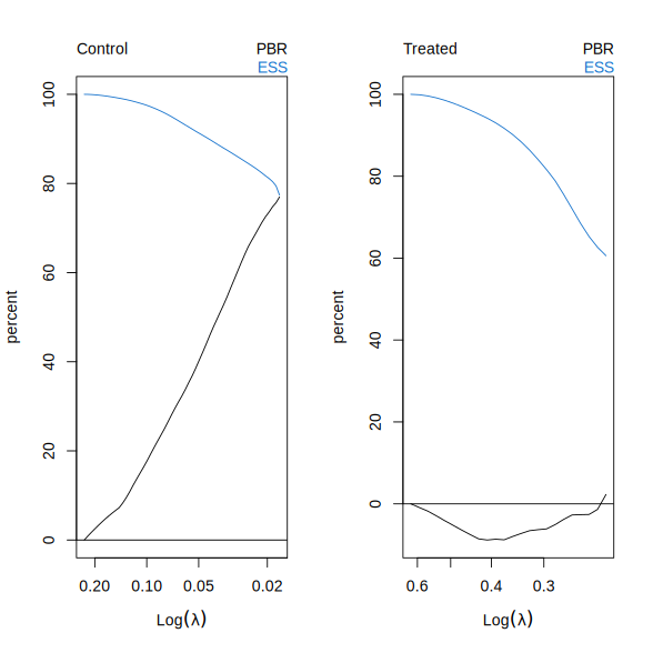
Two quantities are shown, both normalized to percentages. The first is the percent bias reduction (PBR), which measures the reduction in absolute SMD after weighting relative to the unweighted data. The second is the effective sample size (ESS), defined as the squared sum of IPW weights divided by the sum of squared weights, normalized to sum to 100.

Recall that \(\lambda^{\max}\) corresponds to the intercept-only (unweighted) fit. As \(\lambda\) decreases, covariate imbalance is reduced, but at the cost of a smaller effective sample size, reflecting increased concentration of weights on a subset of units.

Individual covariate SMDs can also be visualized at specific values of \(\lambda\) by supplying the lambda argument. Setting lambda = 0 selects the smallest value along the path.

plot(fit, lambda = 0)

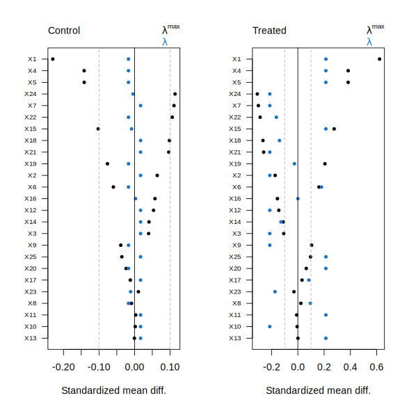
The unweighted SMDs are shown at \(\lambda^{\max}\), while colored points correspond to the weighted SMDs at the selected \(\lambda\). Separate panels are displayed for the treated and control arms, reflecting the fact that distinct propensity score models are fit for each arm in the ATE case. In balnet, SMDs take the form \((\text{weighted mean covariate} - \text{target mean}) ~/~ \text{sd(target)}\).

In this example, the plots suggest limited overlap for the treated arm, indicating that the ATE may not be an appropriate target estimand. Instead, we can target the average treatment effect on the treated (ATT) by setting target = "ATT". In this case, balnet fits a model that aims to balance control covariate means toward those of the treated group.

fit.att <- balnet(X, W, target = "ATT")
plot(fit.att, lambda = 0)

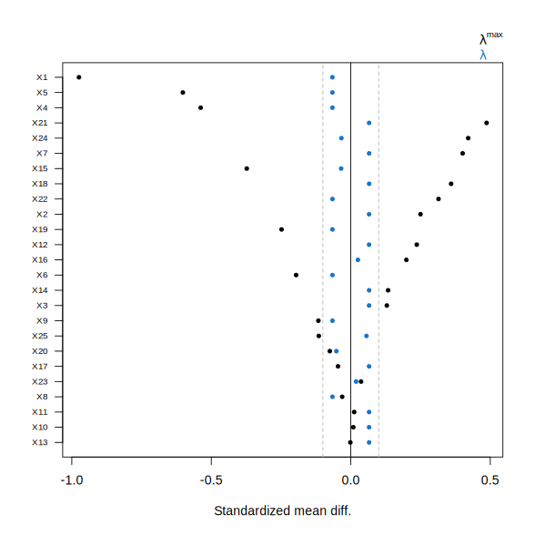
Here, the resulting IPW weights achieve substantially improved balance.

For additional functionality, users are encouraged to consult the documentation for the standard S3 methods provided by balnet, including predict for propensity score prediction and coef for extracting estimated coefficients. On large datasets, we recommend calling balnet with verbose = TRUE to interactively print balance metrics during fitting.